The Horseshoe
In the previous post we watched colour matching turn out to be linear — that matches scale and add like ordinary algebra — and then watched that clean picture crack. Three real primaries cannot match every colour by positive mixture: run the colour-matching experiment on a saturated cyan-green and one of the three knobs goes negative, the red light forced across to the test side because no lamp emits a negative amount. That negative lobe was a genuine embarrassment for anyone trying to standardise colour in 1931. You cannot build a colorimeter that subtracts light, and you cannot tabulate a colour atlas whose own coordinates go negative across half the spectrum without endless sign-juggling. The question Post 4 left on the table is the one this post answers: how do you banish the negativity for good?
The people who did it were a committee. In September 1931, in Cambridge, the Commission Internationale de l’Éclairage — the CIE, a body that one practitioner has affectionately called a bunch of colour nerds, another a bunch of guys in France — sat down to fix a universal coordinate system for colour and engineered the negative lobe out of existence by an act of deliberate fiction. They chose three new primaries with the property that no setting of them ever required a negative coordinate — and the price they paid was that the three primaries are not real. No lamp can emit them, no laser produces them, no star has ever radiated them; they sit outside the set of physically possible colours, three impossible lights chosen precisely because their triangle swallows everything the eye can see. The diagram that fell out of this construction is the most reproduced image in all of colour science: a rounded, tongue-shaped curve, the colours of the rainbow bent into a horseshoe and closed off along the bottom by a straight line of purples that exist in no rainbow at all. Almost every difficulty in the rest of this series is written somewhere on that horseshoe. This post builds it from the ground up.
Four constraints that pin down XYZ
Now to make this precise. The trade the CIE made — real primaries with negative coordinates for imaginary primaries with positive ones — is a change of basis, nothing more. From Post 4 we have the colour solid as a three-dimensional real vector space, and RGB and LMS as two coordinate systems on it, related by an invertible matrix. XYZ will be a third coordinate system, a third basis, and the whole content of the CIE 1931 standard is one specific matrix carrying the Wright–Guild RGB coordinates of Post 4 into a new triple .
A matrix has nine entries. Left unconstrained, the choice would be arbitrary, and the resulting numbers would look magical — a table to be memorised rather than understood. They are not magical. The committee imposed four design requirements, each a linear condition on the entries, and those requirements very nearly pin the matrix down on their own. The textbook payoff of this whole section is that you can watch the matrix assemble itself out of four sentences of intent.
Constraint 2 is a debt this series has been carrying since Post 3. There we met chasing brightness through Purkyně’s garden at dawn — the cone-weighted curve peaking at in the yellow-green — and promised that it would return as the luminance axis of the entire CIE system. This is the payoff. Of all the ways to slice colour into three numbers, the CIE chose the one slicing whose second coordinate means brightness, and the constraint that does it is the bald requirement that one matching function equal on the nose. The luminous-efficiency curve of the twilight flowers is, quite literally, the second row of the matrix.
That second row is worth pausing on. Written out, the photopic weights of the Wright–Guild primaries are , , , and they sum to exactly . Their dominance by the middle term — green carries more than four-fifths of the luminance — is the same fact that makes black-and-white photography legible: strip the colour out of an image and the green channel alone almost reconstructs the brightness of the scene. The line in chromaticity space along which this luminance weighting vanishes has a name out of Greek, the alychne, the “lightless” line, and two of the three imaginary primaries are made to lie on it.
Constraints 1 through 4 are seven linear conditions; the matrix has nine entries; the remaining freedom the committee spent pushing the implied primaries as close to the spectral colours as non-negativity allows, and arranging that the short-wavelength function vanish beyond so the arithmetic of long-wavelength reds stayed clean. What emerges is a single, exact, rational matrix.
Every entry is now legible. The second row is constraint 2, the luminance weights, summing to one. The columns are the new basis vectors written in the old RGB coordinates; that the bottom-left entry is exactly zero is the deliberate choice that kept clean at the red end. The whole transformation is the negative lobe’s cure, and it is nothing but a change of basis, the same kind of matrix that already related LMS to RGB.

The CIE 1931 RGB→XYZ transformation matrix, , set in a clean tabular form with the three Wright–Guild primaries () labelling the columns and the four design constraints annotated row by row: the luminance row (constraint 2) highlighted with its weights summing to unity. A static reference companion to .
The price, promised by the previous post, is now unavoidable. Push the unit basis vectors of XYZ — the pure primary , the pure primary , the pure primary — back through the chromaticity projection we are about to define, and they land at the chromaticities , , : the three corners of a right triangle. None of those three points lies inside the horseshoe of real colour. They are imaginary primaries — colours in the strict technical sense that they have well-defined tristimulus coordinates, but no spectrum produces them, because they sit outside the cone of realisable light. The committee bought positivity with impossibility. You can spend a positive amount of an impossible light, on paper, where you could not spend a negative amount of a real one. We will see the three of them sitting out beyond the horseshoe in a moment, once the horseshoe itself is drawn.
The projection: chromaticity as colour modulo intensity
Colour as we have built it is three-dimensional, and three-dimensional things are awkward to print. The chromaticity diagram is the standard escape: it throws away one of the three dimensions, the one carrying overall intensity, and keeps the two that carry what we ordinarily mean by which colour. The operation that does this is projective, and stating it that way is the cleanest piece of mathematical hygiene in the whole subject.
The defining feature is the denominator. Scaling a colour by any positive factor — turning the same light up or down — multiplies , , all by , and the cancels top and bottom. Chromaticity is therefore colour modulo intensity: the map identifies every point of a ray through the origin with a single point of the plane. A chromaticity is not a colour but an equivalence class of colours, a whole ray’s worth of brightnesses collapsed to one dot. This is why the diagram is two-dimensional, and why a point on it answers “what hue and how saturated” while saying nothing about “how bright.” The third number, the one we divided out, is recovered by carrying along separately — the convention — which is exactly the separation of luminance from chroma that constraint 2 was built to enable, and that we flagged in Post 3 as one of the central design moves of twentieth-century colour science.
To see the boundary of all colour assemble itself, trace a single monochromatic light along the spectrum and watch where its chromaticity lands. The widget below lets you drag the wavelength; the panels read out , , and live, and the moving dot stays pinned to the outer rim of the diagram. Drag from violet at to red at and notice the dot never once steps into the interior.
W-12 — the spectral-locus tracer. Drag the wavelength slider across – and the point traces the outer boundary of the diagram, the spectral locus, labelled with its wavelength; the side panels give the cone responses, the tristimulus values, and the chromaticity. Toggle the view to see the same locus in the more perceptually even coordinates of Post 11. The filled colour inside the diagram is a screen approximation — a real display cannot show most of these chromaticities, a point the horseshoe argument below makes exact.
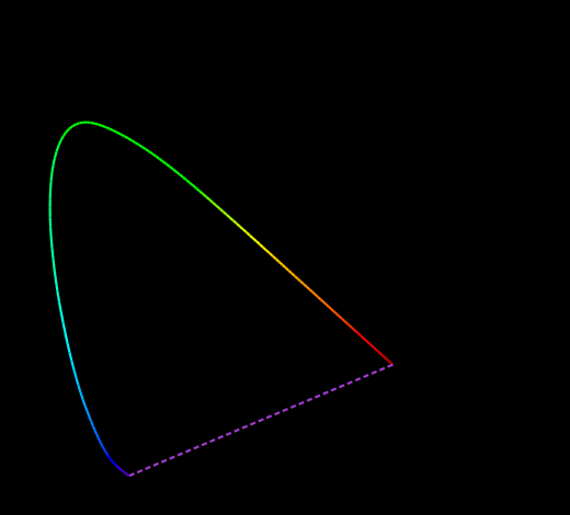
The curve the dot traces is the spectral locus: the chromaticities of the pure single-wavelength lights, the most saturated colours the eye can register. It runs from the deep violet near at , up the left flank to a sharp green tip near around , and down the right side to red near at . Its two ends do not meet. The straight chord closing the gap between the violet and red extremes is the line of purples, and the colours along it — magentas, purples, the vivid pinks — are non-spectral: no single wavelength produces them, they exist only as mixtures of light from the two opposite ends of the spectrum. Purple is the eye’s invention, a colour the rainbow does not contain, manufactured whenever the long-wavelength and short-wavelength cones fire together with nothing in the middle. The closed curve — locus plus line of purples — bounds the gamut of all human colour.
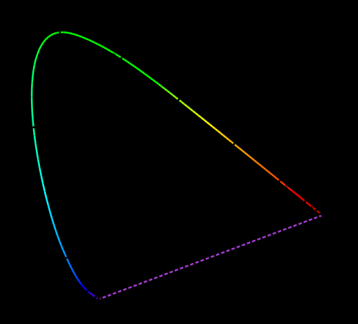
The CIE 1931 chromaticity diagram. The spectral locus is drawn as the curved boundary with wavelength ticks at intervals from to ; the line of purples closes it along the lower-left as a straight chord, labelled non-spectral. The equal-energy white at and the daylight white D65 at are marked. The interior fill is illustrative only — most chromaticities shown cannot be reproduced by the screen displaying them.
Now the imaginary primaries can be shown for what they are. The pure , , basis colours land at , , — three points well outside the horseshoe, forming a right triangle that completely encloses it. That enclosure is the entire point: the triangle of the three primaries contains every visible chromaticity, with room to spare, which is exactly why every colour gets non-negative coordinates. A triangle that swallows the horseshoe must have its corners outside the horseshoe, and a corner outside the horseshoe is an impossible colour. The impossibility is not a flaw in the construction; it is the construction. Pushing primaries deliberately outside the locus to guarantee positive coverage is a move the series will meet again — modern cinema’s ACES working space does it on purpose, with primaries placed frankly beyond the realisable, the XYZ idea taken to its logical end.
The three imaginary CIE primaries , , plotted at , , outside the spectral locus, with the right triangle they span shown enclosing the entire horseshoe of real colour. Two of the three vertices lie on the alychne, the line of zero luminance. The shaded region between the triangle and the locus is the set of tristimulus values with valid coordinates that correspond to no physical light — the imaginary colours that positivity costs.
The horseshoe argument: why no triangle ever covers it
Here is the keystone of the entire gamut half of this series, and it is a one-line theorem about convex sets dressed in the language of colour. Every physical display — every phone, every cinema projector, every television ever built or ever to be built — generates colour by mixing three primary lights, and three real primaries are three points inside the horseshoe. The colours the device can make are exactly the mixtures of those three, which by Grassmann additivity form the triangle with those three points as vertices. The question is whether any such triangle can fill the horseshoe. It cannot, and the reason is geometry alone.
The convexity is itself a consequence of additivity. A mixture of two lights lands, on the diagram, on the chord between their two chromaticities — the diagram is barycentric, a weighted average — so any chord between two visible chromaticities is filled with visible colours, which is the definition of a convex set. The gamut is thus the convex hull of the spectral locus. A triangle inscribed in a convex region with curved boundary cuts that boundary with three straight chords, and each chord slices off a sliver of the region lying outside the triangle but inside the gamut. Those slivers are the colours the device cannot reach. They are concentrated along the curved flanks of the horseshoe — the saturated greens and cyans where the locus bulges out most — precisely the region where the cyan-green negative lobe appeared in Post 4. The negative lobe and the unreachable gamut are the same fact wearing two costumes: the locus curves away from any triangle of real primaries, so naming its colours in those primaries requires either negative coordinates or imaginary corners.
One honesty note is owed, because a careful book does not overstate its theorems. The spectral locus produced by the standardised 1931 matching functions is not perfectly convex; it has two slight pockets of concavity, one near and one in the deep blue between roughly and , almost certainly artefacts of the Wright–Guild reconstruction rather than features of the eye. They amount to a small fraction of a percent of the gamut area and are invisible to any practical colorimetry. The gamut-limitation conclusion does not depend on perfect convexity: a triangle’s straight edges chord across the curved bulk of the locus whether or not two tiny pockets are strictly convex, and the unreachable region survives intact.
The widget below makes the theorem operable. Toggle on the standard display gamuts and watch each one sit as a triangle strictly inside the horseshoe, its three straight edges chording across the curve and leaving the saturated rim uncovered.
W-13 — the chromaticity diagram with overlayable display gamuts. Toggle sRGB/Rec.709, DCI-P3, and Rec.2020 (and the wide working spaces) on and off; each appears as a labelled triangle, distinguished by line style rather than colour alone. Switch the diagram between and the more even coordinates, and click any point to read its chromaticity and which gamuts contain it. ACES AP0 visibly poke its corners outside the locus — the same imaginary-primary move as XYZ. Triangle fills are hatched, not solid, because the screen cannot truthfully display colours its own gamut excludes.
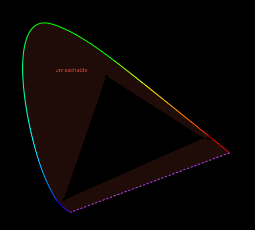
The sRGB/Rec.709 triangle overlaid on the spectral locus, its three straight edges chording across the curved boundary. The crescents of gamut lying outside the triangle but inside the horseshoe — concentrated in the saturated greens and cyans along the upper-left flank — are shaded “unreachable by this device.” A static companion to W-13.
This is a permanent fact about every future display, not a limitation of present technology. When a later post shows Rec.2020’s straight blue-green edge cutting across the locus and missing the most saturated azures, that is this theorem made physical — no future primary, however pure, escapes it, because the obstruction is the curvature of the boundary, not the quality of the lamps. There is a consoling footnote: most of the colours stranded outside a good display’s triangle are extreme spectral colours that rarely occur in ordinary scenes, the province of lasers rather than of light reflecting off objects, which is why an sRGB screen looks convincing despite covering only a third of the diagram.
A second honesty note, which we will cash out later. Euclidean distance on this diagram is badly misleading: equal steps in correspond to wildly unequal perceptual differences, the green region stretched and the blue compressed, the way a Mercator map distorts area. The diagram is a faithful map of what is reachable and a treacherous one of how different two colours look. Quantifying that treachery — MacAdam’s ellipses, the empirical proof that the plane is not perceptually flat — is a later chapter; for now, read the horseshoe for its boundary, not its metric.
One space, many bases
Step back from the diagram and the larger structure is plain. LMS, RGB, and XYZ are three coordinate systems on one three-dimensional space — the image of the projection from spectra to that Post 4 built. The same room, measured against three different sets of walls. Moving between any two is a single invertible matrix, and composing the moves just multiplies the matrices.
A linear change of basis has two properties worth naming because the diagram depends on both: straight lines stay straight, and the origin stays fixed. The first means a chromaticity line — the image of a mixture — survives the LMS-to-XYZ change unbroken, so the barycentric mixing rule that gave us convexity holds in every one of these coordinate systems. The second means the black point is shared. The widget below shows the same cloud of colours and the same spectral-locus curve sitting in each basis in turn, morphing as you switch the target, the matrix displayed acting on a highlighted vector so you can watch a single colour’s coordinates transform.
W-11 — the change-of-basis visualiser. Orbit a three-dimensional view of the spectral-locus curve and a handful of sample colours; pick the target basis (XYZ, CIE-RGB, or linear sRGB) from the dropdown and the cloud morphs to its new coordinates while the active matrix is shown acting on a highlighted vector. Straight lines stay straight and the origin stays put — the two signatures of a linear map — so the mixing geometry is preserved through every basis. On a phone the morph is replaced by a labelled before/after pair.
There is one basis change in this family that is not what it first appears, and it is the subtle point the series must take a position on. Going from XYZ to LMS — from the historical coordinates back to the physiological ones, the actual cone responses — sounds like it should be a single fixed matrix, the way RGB-to-XYZ is the single fixed matrix . It is not. There is no canonical XYZ-to-LMS matrix, and the reason is structural.
The 1931 functions were reconstructed from Wright and Guild’s observers and the 1924 luminance curve; the cone fundamentals were derived decades later from different data — Stiles–Burch wide-field matches and cone-isolation measurements on dichromats of known genotype. The two reconstructions do not land on the same three functions, and three functions that span a different subspace cannot be reached by any change of basis. So the literature carries a small zoo of matrices, each a best fit under different criteria: the Hunt–Pointer–Estévez matrix built for chromatic-adaptation modelling, the spectrally sharpened Bradford matrix used inside ICC colour profiles, and the CAT02 matrix at the heart of the CIECAM02 appearance model. The first is a genuine attempt at cone fundamentals; the latter two are deliberately not cone spaces at all — their axes are narrowed beyond physiological cones to make white-point adaptation behave, a trick we will return to when we adapt colour across illuminants.
The book must choose, and state the choice. We take the Hunt–Pointer–Estévez matrix, normalised so that D65 maps to , as the default LMS:
When a later post uses a different matrix — Bradford or CAT02 for adaptation — it is because the engineering goal there is sharpening, not physiology, and we will say so each time rather than pretend one matrix is canonical. The widget below makes the non-uniqueness concrete: pick a colour, then switch conventions and watch its shift under each matrix while the implied cone primaries move on the diagram.
W-15 — the XYZ→LMS matrix playground. Choose a convention from the dropdown — Hunt–Pointer–Estévez, Bradford, CAT02, or the physiological CIE 2006 set — and the displayed matrix and the resulting of a draggable test colour update together, plotted side by side so the disagreement is visible. The implied LMS “primaries” shift on the chromaticity diagram with each choice. Bradford and CAT02 are sharpened adaptation bases, not literal cone spaces; they reappear in that role in Post 6.
The optimal-colour solid: colour is a volume
The horseshoe tempts a reader into thinking of colour as a two-dimensional thing, a shape on a page. It is not. We divided out intensity to get the diagram, and intensity is a real dimension; the full set of realisable colours is a volume in three-space, and its shape is more interesting than the triangle-versus-horseshoe story lets on. The question that fixes the volume is the one Erwin Schrödinger asked in 1920, before he had a wave equation to his name: among all the surface colours of a given chromaticity, which is the brightest the laws of physics permit?
A surface colour is a reflectance function , the fraction of incident light the surface returns at each wavelength, constrained by physics to lie between and . The colour it shows under a given illuminant is the tristimulus integral of the reflected light. Schrödinger’s insight, made rigorous by David MacAdam in 1935, is that the reflectances achieving the maximal luminance for each chromaticity — the optimal colours, the boundary of what surfaces can do — are not smooth curves but sharp two-transition step functions: reflectance is either or at every wavelength, switching exactly twice across the band. A surface gets the most luminance into a hue by reflecting all the light it can in a band and none outside it — a rectangular spectral window. Sweep the two transition wavelengths over all positions and you trace out the boundary of the realisable-colour solid, the MacAdam limits.
The convexity here is the same additive convexity as before, now in three dimensions: any mixture of realisable colours is realisable, so the realisable set is convex, and the optimal two-transition colours are its extreme points. Rotating the solid shows what the flat diagram hides — that a display’s gamut is a small box nested deep inside a fat, bulging object-colour solid, and that the chromaticity triangle is merely the solid’s shadow seen from directly above.
W-14 — the visible-gamut three-dimensional solid. Orbit the optimal-colour (MacAdam-limit) solid and the sRGB gamut box nested inside it; toggle the spectral-locus curve, switch the coordinate space among XYZ, CIELAB, and OkLab, and snap to canned viewpoints (top-down recovers the chromaticity horseshoe; side-on shows the luminance axis). The surface colours are screen approximations of colours the screen mostly cannot show. On a phone this is a static labelled render.
The optimal-colour (MacAdam-limit) solid rendered in XYZ, with the sRGB display gamut shown as a small box nested inside it and the spectral-locus curve running up its outer surface. The solid’s pointed top and bottom are the bright yellows and dark blues; its widest girth is the mid-luminance band. A frozen three-dimensional companion to W-14, and the proof that the chromaticity triangle is a shadow of a volume.
This convex solid is the set you cannot leave by mixing lights within it — every combination of realisable colours stays realisable, which is precisely what convexity means. That closure has a consequence the series saves for its final post: if there is a colour sitting outside this solid, no light and no surface and no display can ever produce it, and the only way to reach it would be to bypass light entirely and stimulate the retina directly. There is such a colour. We will meet it at the end.
Metamerism: two spectra, one colour
We close where Post 4 began, on the projection itself, now seen from the far side. The map from the infinite-dimensional space of spectra to the three-dimensional space of colour has an enormous kernel — an infinite-dimensional subspace of spectra the eye reads as identical to darkness — and that kernel is the whole reason colour reproduction is possible and the whole reason it sometimes fails. Two spectra produce the same colour exactly when their difference lies in . The technical name for an element of that kernel is a metameric black: a non-zero spectral distribution that the three cones integrate to zero, a pattern of light the eye cannot tell from no light at all.
This is the collapse of Post 2 made fully visible. Three cones read a continuum of wavelengths out as three numbers; a projection that drastic — uncountably many input dimensions onto three — must be many-to-one, with whole infinite-dimensional families of spectra crowding over each point of the image. Metamerism is not a quirk of pigments or a defect of any particular eye; it is the generic and unavoidable consequence of projecting an infinite-dimensional space onto a three-dimensional one. Maxwell’s tartan ribbon worked because his three filtered plates kept exactly the three projections the cones keep, so the reproduction and the original differ by a metameric black and the eye cannot separate them. The same fact runs the entire reproduction industry: every screen you have ever looked at lies about the spectrum and tells the truth about the colour, and you cannot tell, because the lie lives in .
The widget below is the grand finale of “matching,” the thing the last two posts have been building toward. Construct one spectrum by dragging its handles, then construct a visibly different second spectrum and lock it to share the first’s cone responses. The two spectral plots will look nothing alike; the two swatches will be indistinguishable; the single chromaticity dot will sit under both.
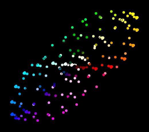
W-10 — the metameric mixer. Shape one spectrum with the amplitude handles, then a second spectrum , and engage “lock to metamer”: the second is projected onto the affine subspace sharing the first’s by adding a metameric black, so the two curves diverge in shape while their cone responses, their , and their chromaticity coincide and . The two swatches sit on a fixed grey card for honest comparison; if no non-negative metamer exists for the chosen handles, the widget says so rather than faking one.
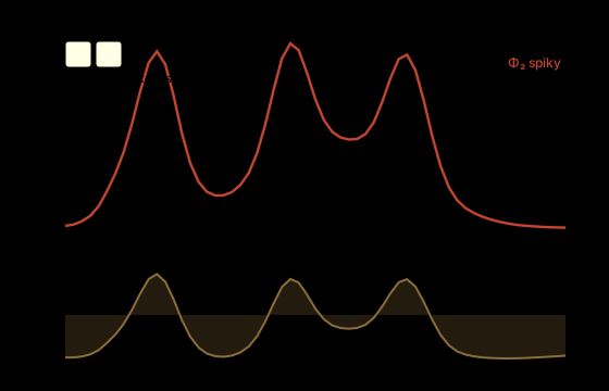
Two visibly different spectral power distributions plotted on the same axes — one smooth and broad, one spiked and narrow — annotated with their identical values, beside two colour swatches that are indistinguishable on a grey surround. Their difference, plotted below, is a metameric black: a spectrum that crosses zero such that all three cone integrals vanish. A static companion to W-10.
One last clause carries a warning the series will collect on twice. A metameric match holds only under a fixed illuminant: two spectra that match under daylight can split apart under tungsten, because changing the light changes which spectrum reaches the eye and the difference need no longer lie in . This is why a colour “match” is always a match under some light — the fine print of Post 2’s four senses of “match” — and the failure mode of every metameric reproduction. It is also the formal root of an illusion we will not be able to resist: when the same pixels look like two different colours under two different inferred lights, the dress that broke the internet, the brain is solving exactly the ambiguity this clause names. And because we so carefully kept separate as luminance, we have a standing reminder that luminance is not the same as perceived brightness — a saturated colour can read as brighter than a white of equal — the seam between what the matrix measures and what the eye reports.
The committee in Cambridge set out to banish a minus sign and ended by drawing the boundary of all colour. The horseshoe is what positivity costs and what positivity buys: a universal coordinate system, three impossible primaries, a curved boundary no real display will ever reach, and a three-number address for every colour that any two spectra can share. We have the map. We have not yet asked what fills it — what makes a flame red and the noon sky white, and why “white” turns out to be a moving target rather than a fixed point.