Brown, Moonlight, and the Island of the Colour-Blind
In the previous post we found the collapse that makes colour: three kinds of cone in the fovea, and a spectrum read out as three numbers, so that two lights “match” when they land on the same triple even if their spectra differ wildly. We also left a loose end hanging — that the cones rule the bright, central few degrees of vision, but a different receptor takes over in the dark, one we named and then walked past. If colour is three numbers from three cones, what happens to it at the edges: when a cone is missing, when there might be a fourth, and when the light falls so low that the cones go quiet altogether?
Start at the most extreme edge. In the Pacific, a thousand miles north of New Guinea, there is an atoll called Pingelap: a ring of coral barely two square kilometres of dry land, home to a few hundred people. Around 1775 a typhoon named Lengkieki swept the atoll and killed all but a score of its inhabitants, and in the generations of close intermarriage that followed, a rare recessive gene surfaced and spread. Today something like one in twelve Pingelapese is born with complete achromatopsia — not red-green confusion, but no functioning cones at all. They see the world through rods alone: in shades of grey, at low resolution, and dazzled to near-blindness by ordinary daylight. The neurologist Oliver Sacks (1933–2015), who sailed there in 1994, found a community that had built itself around the condition rather than against it. The achromats, called maskun — “not see” — fished at dusk and by torchlight when their rod-rich eyes outperformed everyone else’s, wove by feel, and read the reef in a register of brightness and texture the rest of us never learn. Sacks titled the book that came out of the trip The Island of the Colourblind, and the phrase has stuck.
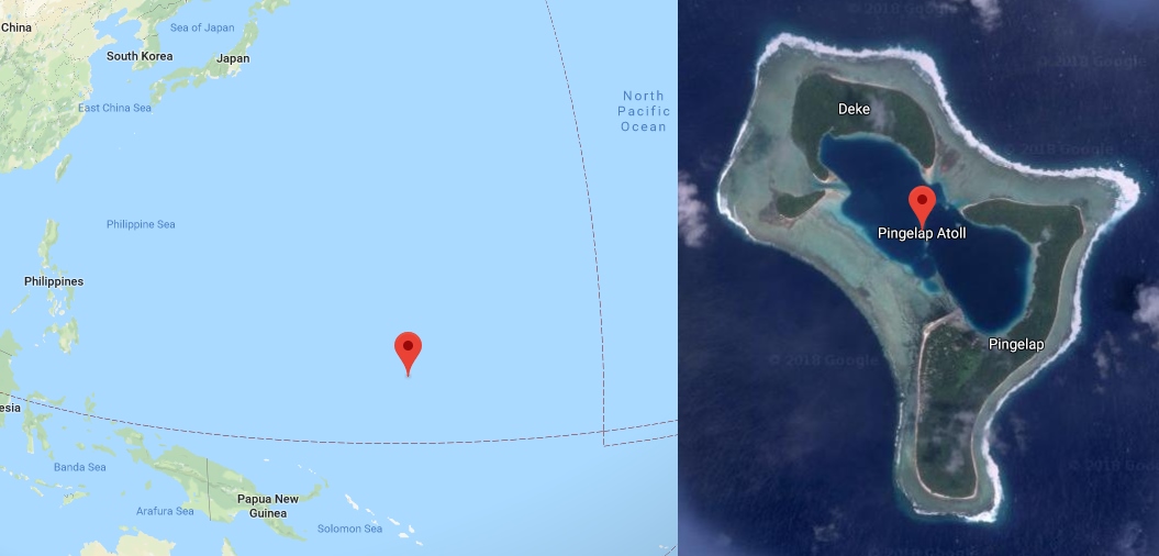
Pingelap atoll — a ring of coral barely two square kilometres across in the Eastern Caroline Islands, a thousand miles north of New Guinea. The 1775 typhoon Lengkieki cut the population to about twenty survivors; in the generations of close intermarriage since, complete achromatopsia surfaced and spread, until roughly one islander in twelve is born seeing no colour at all.
Pingelap is the limiting case of a much broader truth, and a useful one to hold while we work outward from it. The story this post tells is that the three cones of the last post are not a fixed, universal apparatus. They vary from person to person; they can go missing, singly or together; there are hints of a fourth; and even in a single normal eye, the whole system rearranges itself as the sun goes down. Colour, even as a count of dimensions, is not quite the constant the last post made it seem.
A band, not a point
Begin with the variation that hides inside “normal.” The cone fundamentals from the last post — the curves , , the standard observer integrates against — are an average. The pigment in your L cones is a protein, opsin, built from a recipe written in a gene, and the gene comes in variants: a single amino-acid swap at one site (position 180, serine for alanine) shifts the cone’s peak by a few nanometres, and roughly half the population carries each variant. Two people with textbook-normal colour vision can therefore be running slightly different curves, and at the colour-matching experiment of the next post they will dial a red-green mixture to visibly different settings against the same fixed yellow, each certain they are right.
The cleanest analogy is in taste. Whether coriander reads as citrus or as soap is largely set by receptor-gene variants; so is whether a synthetic musk is overpowering or undetectable, whether Brussels sprouts are pleasantly bitter or inedible. These are receptor polymorphisms, the same kind of small genetic dial that nudges an L cone three nanometres along the spectrum. Nobody with the soap variant is tasting coriander wrong; they are tasting a different molecule’s worth of signal. “Normal colour vision” is the same — not a point but a band, a cloud of slightly different observers around the standard one.
This matters more than a curiosity, because it cashes out one of the four senses of “match” we defined last time. A match to me — two spectra that hit my particular cones identically — need not be a match to you, and the gap is not error or imprecision. It is the literal physical fact that we integrate the spectrum against different curves. Hold that thought; it is the small everyday version of the dramatic failures that arrive when a cone is not merely shifted but gone.
What dichromats lose
The opsin genes that build the L and M cones sit side by side on the X chromosome, and they are nearly identical — ninety-six to ninety-eight per cent the same DNA, the residue of a gene duplication in our primate ancestry maybe thirty million years ago. That near-identity is exactly what makes them fragile. In the shuffling of meiosis, two stretches that similar can misalign and cross over in the wrong place, and the array that results can be missing a gene, carrying an extra one, or holding a hybrid — a chimera, half L and half M, whose peak sensitivity lands somewhere in the gap between the two.
What the eye does with that determines which of two failure modes you get. If a cone class is merely shifted — an L gene replaced by a hybrid peaking a little closer to M — the eye still has three channels, but two now sit so close that the difference signal colour lives in is feeble. This is anomalous trichromacy: three numbers, but a flattened, low-contrast space with reds and greens muddied rather than lost. If a cone class is absent — no working L pigment, or no M, or (far more rarely, from a different chromosome) no S — a whole axis is gone, and the eye is a genuine dichromat, reading the world in two numbers instead of three.
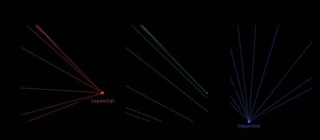
Dichromat confusion lines on the chromaticity diagram. Each pencil of lines radiates from a copunctal point — the chromaticity that would have excited only the missing cone — and every colour lying on one line is indistinguishable to that dichromat. Protanopia, deuteranopia, and tritanopia each have their own copunctal point and their own family of confusion lines. The static geometry behind the simulator below.
The arithmetic of who is affected falls straight out of the genetics. The L and M genes are on the X chromosome, the defects recessive, and men have only one X — so one faulty array suffices in a man, while a woman needs two. Run the Hardy–Weinberg bookkeeping on an allele frequency near eight per cent and you get about one man in twelve of European ancestry with some red-green deficiency, dichromacy and anomalous trichromacy together, against well under one woman in a hundred. The S-cone gene sits on chromosome 7 and is far more stable, so tritan defects are rare by comparison. Around five per cent of all men, then, carry the same single quirk: the L and M genes are too alike for their own good.
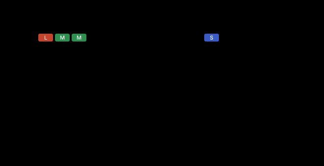
Why the arithmetic is so lopsided. The L and M opsin genes sit head-to-tail in a tandem array on the X chromosome, so red-green deficiency is X-linked: a man, with his single X, needs only one faulty array, while a woman needs two. The S-cone gene sits on chromosome 7 — autosomal, and far more stable — which is why tritan defects are rare and fall on men and women alike.
It is worth seeing what that collapse from three dimensions to two actually does to a scene, rather than only asserting it. Pick a deficiency type and a severity below and watch the chromaticity diagram, and a photograph, fold along the confusion lines.
W-06 — the colourblindness simulator. Pick protan, deutan, or tritan and slide the severity from anomalous trichromat toward full dichromat; the right panel shows the simulated view beside the original, and the caption names what converges. The simulation approximates how a scene looks to a trichromat who has lost an axis — not a literal window onto another mind’s experience.
The thing to notice is which pairs of colours march together as the severity climbs. For a protan or deutan, reds and greens slide toward a common muddy yellow-brown; the two hues a trichromat finds most opposite become, for the dichromat, the same. This carries a practical stake, one a film colourist will tell you without prompting: never hang a shot on a red object popping out of green foliage. To you the red coat against the hedge is the most legible thing in the frame; to the one man in twelve watching, if coat and leaves share a brightness, the coat is simply not there. Redundant cues — brighter, or moved, or a different shape — are not an accessibility nicety but the only way to be sure the information survives the journey through a two-dimensional eye.
The same fact, run in reverse, is the engineering trick behind the test that diagnoses the condition. If you want to build a figure that a dichromat cannot see, you paint it in colours that differ only along the axis they have lost, while holding the brightness constant so no luminance edge gives the figure away. To a trichromat the figure stands out in hue; to the matching dichromat it dissolves into its background. That is the whole principle of the pseudo-isochromatic plate, invented by Shinobu Ishihara (1879–1963) in 1917 when the Imperial Japanese Army asked him for a way to screen conscripts. Toggle a deficiency on the plate below and watch the numeral appear or vanish.
W-07 — an Ishihara-style plate (original, illustrative, not a clinical instrument). The numeral is carried by hue at near-equal luminance; toggle protan, deutan, or tritan simulation and the figure that a trichromat reads clearly drops into the noise for the matching dichromacy. The dots are generated, not the copyrighted official plates.
Pingelap: a world without hue
Now return to the atoll, because Pingelap is what happens when the collapse goes all the way. Protanopia and deuteranopia knock out one axis and leave a two-dimensional colour world — diminished, but still colour. Complete achromatopsia, the maskun condition, knocks out all three cone classes. What remains is the rod system alone, and we are about to spend the rest of this post on what that system can and cannot do, but the headline is simple: it is one receptor, and one receptor cannot make colour at all.
The reason is the dimension-counting we have been doing. Colour lives in the ratio of responses across receptor classes — the gap between and , the gap between and the rest. A rod reports one number, an intensity; a single number can be high or low but cannot be red. Any two lights that drive the rods equally are identical, full stop, so the rod-only eye is a one-dimensional colour space — which is no colour space at all, only a scale from dark to bright. The achromat lives along Aristotle’s old line from the first post, white to black with the hues erased — except this is not a discarded theory but a way of seeing that some people are born into.
And rods come with a second cost, the one that shapes daily life on the atoll. Rods are built for sensitivity, not for daylight; they saturate and shut down when the light is strong, the way an over-gained microphone clips. With no cones to take over in the bright, the achromat in noon sun is not merely colour-blind but nearly blind, flooded and dazzled, squinting through a glare the rest of us never feel. Hence the photophobia Sacks recorded, and hence the inverted clock of Pingelapese life — the achromats most at ease at dusk, fishing the flying-fish runs by torchlight, while the trichromats’ cones were failing them and the rod-rich maskun eyes were just coming into their own. A whole culture organised, quietly, around which receptor works when.
The fourth cone that mostly isn’t used
If subtracting a cone subtracts a dimension, the symmetric question is irresistible: can you add one, and gain a dimension? The answer is a careful and instructive “almost never, but in principle yes, and the bookkeeping matters.”
Recall the recombination that makes hybrid genes. A woman has two X chromosomes; she can carry a normal L–M array on one and a hybrid array on the other, and because one of the two X chromosomes is switched off at random in each cell early in development, her retina ends up a mosaic — some cones built from the normal array, some from the hybrid. If the hybrid’s peak sits far enough from the standard L and M peaks, she is walking around with four spectrally distinct cone pigments: S, M, L, and a fourth, call it L′, a dozen nanometres off L. The genetics is not exotic; the same X-linked shuffle that gives men colour blindness gives their mothers and daughters this. A straightforward count suggests something like one woman in eight of European ancestry carries four pigments.
Here is where precision earns its keep, because the popular version of this story is badly overcooked. Carrying a fourth pigment is potential tetrachromacy: the receptor is there. Whether it does anything is a separate question entirely, and a harder one. To use a fourth receptor as a fourth colour dimension, the eye needs more than the cone — it needs post-receptoral wiring that takes a fourth independent difference and carries it upstream as its own signal. The dimensionality of colour vision is not the number of pigments; it is the rank of the whole channel, receptors plus the neural circuit that reads them.
Two decades of patient work by John Mollon at Cambridge and Gabriele Jordan tested carrier after carrier, and found that almost all of them — though they demonstrably carried the fourth pigment — behaved in the lab as ordinary trichromats. The substrate was there; the extra dimension was not being read. Then in 2010 they reported a single exception, a woman labelled cDa29, who in a demanding forced-choice test — three colour patches flashed quickly, two of them spectrally identical, one differing only along the putative fourth axis — picked the odd one out on every trial, where a trichromat could only guess. One confirmed strong tetrachromat, out of the dozens carefully screened.
The honest summary is the unhyped one. Potential tetrachromacy is common; functional tetrachromacy is, on the present evidence, vanishingly rare, and what cDa29 actually experiences is something nobody — including cDa29, in any words a trichromat can receive — has been able to convey. (Tetrachromacy is, by contrast, the ordinary condition for birds, which routinely carry a fourth cone peaking in the ultraviolet, and which therefore see patterns on flowers and feathers that are simply invisible to us.)
The reason to be precise here is not only scientific manners. It is that a real fourth channel would break something structural in everything this series builds next. The whole edifice of chromaticity — the horseshoe diagram of the fifth post, every gamut triangle, every flat map of colour we are about to draw — rests on colour being three-dimensional, so that chromaticity, colour with brightness divided out, is two-dimensional and fits on a page. A genuine tetrachromat’s colour space is four-dimensional; her chromaticity is not a region of the plane but a surface in three-space, a 2-sphere rather than a 2-disc. Every planar diagram in the rest of this series is, strictly, a diagram of our colour vision, three pigments wide. For cDa29, the page is one dimension short.
The birth of brown
Set the receptor count aside now — back to three, the ordinary case — and notice something we have been quietly suppressing. Every “colour” we have discussed has really been a chromaticity, a question of which wavelengths in what ratio, with the overall intensity divided out. But intensity is not nothing. It is a second axis, and to feel how much it carries, consider a colour that does not appear anywhere in Newton’s spectrum at all.
There is no brown in the rainbow. Run through the spectral colours from the first post — red, orange, yellow, green, blue, violet — and brown is nowhere among them; there is no wavelength of brown light, no laser you could tune to it. And yet brown is utterly ordinary: wood, soil, coffee, bread, skin, the most domestic colour there is. Where does it come from, if not from the spectrum?
It comes from darkness. Take a patch of saturated orange — fixed chromaticity — and lower only its luminance while the brighter things around it stay bright, and somewhere along the way the name changes under you: orange, then a deepening ochre, then unmistakably brown, then near-black. Nothing about the mix of wavelengths changed; only the intensity, and only relative to the surround. Brown is dark orange — a colour that exists only as the dim member of a bright scene, which is exactly why a single light considered alone can never contain it.
W-04 — luminance and the birth of brown. Fix the chromaticity at orange and drag the luminance down from full; the swatch slides orange → brown → black with the chromaticity never changing, and a fixed full-luminance swatch beside it supplies the bright surround that makes “brown” read as brown. Scaling happens in linear light, then encodes to the screen; the “brown” label is perceptual and depends on that surround.
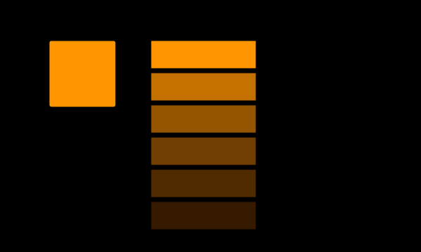
The orange-to-brown-to-black luminance ladder: a single chromaticity sampled at decreasing luminance , the perceived-colour name annotated at each rung (saturated orange, ochre, brown, near-black). The chromaticity coordinates are identical at every step; only changes. The static companion to W-04.
This is the entering wedge of a much larger idea. Colour has been three numbers, but those three numbers split naturally into two about hue and saturation and one about brightness, and the brightness axis turns out to carry an astonishing share of the information — the whole legibility of a black-and-white photograph is proof that you can throw the other two away and still read the world. The clean separation of that one luminance axis from the two chromatic ones is one of the central design moves of twentieth-century colour science, and it is the explicit goal of the transformation we build in the fifth post. For now, the lesson is just that intensity is a real and independent dimension, and that brown is its most charming witness.
When the rods take over
Which brings us, finally, to the receptor we named in the last post and then deferred — the rods — and to what becomes of colour when the light gets low enough to hand vision over to them.
We owe the rods a proper introduction, because the last post gave them only a sentence. They outnumber the cones enormously — something like ninety-two million rods to under five million cones — absent from the very centre of the fovea but blanketing the periphery. They carry a single pigment, rhodopsin, peaking around 498 to 507 nanometres, in the blue-green between the S and M cone peaks. Being a single pigment, the rod system is, on its own, exactly as colour-blind as the Pingelap achromats: one number, no ratios, no hue. What the rods buy with that sacrifice is sensitivity — they respond down to a handful of photons, far below anything the cones can register — and a different spectral tuning. Those two facts together produce the most quietly strange phenomenon in everyday vision.
Now to make this precise. Brightness, as the eye reckons it, is not a flat sum over wavelengths; it is the spectrum weighted by a sensitivity curve, and that curve is not fixed. With the cones in charge it is the photopic luminous-efficiency function , peaking at 555 nm in the yellow-green — roughly the sum of the L and M cone fundamentals, which is why the spectrum looks brightest there. With the rods in charge it follows rhodopsin instead: the scotopic function , peaking near 507 nm, shifted toward the blue. The apparent brightness of a light with spectral power is, in each regime,
and because and peak nearly fifty nanometres apart, the same two lights can rank differently in brightness depending on which curve is doing the weighting.
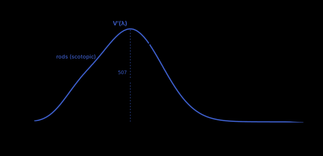
The two luminous-efficiency curves: photopic , peaking at (cone-mediated), and scotopic , peaking near (rod-mediated). The roughly fifty-nanometre gap between the peaks is the Purkinje shift made quantitative — long-wavelength reds weighted heavily by but barely by . The static companion to W-05.
That nearly-fifty-nanometre gap is the whole phenomenon, and it has a name and a date. In 1825 the Czech physiologist Jan Evangelista Purkyně (1787–1869) was walking in his garden at dawn and noticed something he could not unsee. The red flowers that had been the brightest things in the bed by daylight were now the dimmest, nearly black; the blue flowers, easy to overlook at noon, were the ones that glowed. Nothing about the flowers had changed — only the light level, and with it the curve: as vision slid from cone-weighted toward rod-weighted , the long-wavelength reds the rods barely register sank toward black, while the short-wavelength blues, sitting near rhodopsin’s peak, held and even gained. This is the Purkinje shift, and the arithmetic is stark: a red at 620 nm has photopic efficiency around but scotopic around , while a blue at 470 nm runs the other way, photopic against scotopic — so the blue flower is some fifty times brighter to the rods than the red.
You can run Purkyně’s garden on a slider. Drag the ambient level from noon down toward moonlight and watch the red and blue flowers trade places, and the effective brightness curve slide from one peak to the other.
W-05 — the Purkinje shift. Drag the ambient level from photopic (noon) through mesopic to scotopic (moonlight); the line plot morphs the effective luminous-efficiency curve from (peak ) toward (peak ), and the red and blue flowers swap brightness order as it moves. At full scotopic the swatches desaturate toward grey, because rod-only vision has no hue — the honest end state, not vivid flowers in the dark.
Between the two regimes lies the mesopic range — the luminances of dusk, of a lamplit room, of most night driving — where rods and cones both contribute and there is no single clean efficiency curve, only a blend that shifts with the ambient level. This is the regime of the “blue hour,” the interval after sunset when the sky has gone a deep saturated blue and the world looks faintly luminous and strange: partly the spectrum of the twilit sky, but partly the Purkinje shift catching you in the act, your blues brightening and your reds dropping away as the rods come up. The colour of late evening is, in part, your own retina rearranging itself.
There is one more thing to say about , and it is a promise rather than a payoff. This curve will not stay confined to the story of twilight. When we build the chromaticity diagram in the fifth post, we will need to choose, out of all the ways to slice colour into three numbers, the one that makes a single axis mean brightness — and the constraint that does it is precisely that one of the colour-matching functions be set equal to , exactly. The luminous-efficiency curve of Purkyně’s flowers becomes the luminance axis of the entire CIE system. And later still, when we ask how brightness gets measured rather than merely felt, will define the candela itself — the SI unit of luminous intensity is built by weighting raw radiometric power against this very curve. A function we met chasing a garden at dawn underwrites both the geometry of colour space and the numbers on a light-meter. We will earn both claims when we reach them.
Three edges, then, and one lesson behind all of them. Subtract a cone and a dimension goes with it, down to the rod-only line where colour cannot exist; add a cone and, in rare wiring, a dimension might appear, breaking the flatness of every diagram to come; and even in one unremarkable eye, drop the light and the whole weighting of brightness slides out from under you. The three numbers of the last post were never a fixed instrument. They are a configuration — one common setting of a system that varies between people, fails in structured ways, and reconfigures itself with the sun.
Next: why three carefully chosen lights can be mixed to match almost any colour you can see — and the strange necessity of mixing in a negative amount of red.