Maxwell's Tartan Ribbon
In the previous post we watched the three numbers of colour bend and break at the edges of vision — a cone shifted, a cone gone, the whole weighting of brightness sliding out from under us as the light fell. Underneath all of it sat the same machinery from Post 2: three kinds of cone read a spectrum out as a triple, and two lights “match” when they land on the same triple. That leaves the practical question the whole technology of colour turns on. If a light is only ever three numbers to the eye, then three suitably chosen lights ought to be enough to forge any of those numbers — to manufacture a match for almost anything you can see. Why should that work, exactly when does it fail, and what does the failure look like?
On the evening of 17 May 1861, in the lecture theatre of the Royal Institution in London, a thirty-year-old Scottish physicist set out to answer the first part of that question in front of an audience. James Clerk Maxwell (1831–1879) had brought a small bow of tartan ribbon, and three black-and-white photographic slides of it, each shot through a different coloured liquid: a red, a green, a blue. He handed the slides to the photographer Thomas Sutton — the man who had built the first single-lens reflex camera — and had him project all three at once onto a screen, each through the same colour of filter it had been taken through. The red record went back up through red light, the green through green, the blue through blue. Where the three overlapped, a recognisable colour image of the ribbon swam into view: the first colour photograph ever made, conjured out of three grey pictures and three coloured lamps.
The tartan ribbon
The principle is worth slowing down on, because the entire reproduction industry is a footnote to it. A scene reflects some spectral power distribution toward the camera — an arbitrary, wiggly function of wavelength, in principle carrying infinitely much information. Maxwell did not record that function. He could not have; no plate stores a whole spectrum. Instead each of his three exposures multiplied the incoming light by a filter’s transmission curve and integrated, collapsing the spectrum at every point of the image down to a single number — how much got through the red filter, how much through the green, how much through the blue. Three filtered exposures, three numbers per point. The wiggly function was thrown away and three weighted sums were kept in its place.
That should, by any naive accounting, be a catastrophe. You have discarded almost everything about the light. And yet projected back through the matching filters the three numbers reconstitute a believable colour — because the eye that judges the result performs the very same reduction. The cone system, as we built it in Post 2, also collapses to three numbers, the triple . If Maxwell’s three filter-and-plate responses span the same possibilities the three cones span, then any spectrum and its three-number reproduction excite the cones identically, and the eye cannot tell them apart. The reproduction is not a copy of the light. It is a metamer of the light — a different spectrum chosen to land on the same triple — and metamerism, the apparent defect we met as the gap between two senses of “match,” is here the engineering principle that makes colour photography conceivable at all. Maxwell’s grey plates threw away the spectrum and kept exactly the three projections the eye keeps. That is why it works.
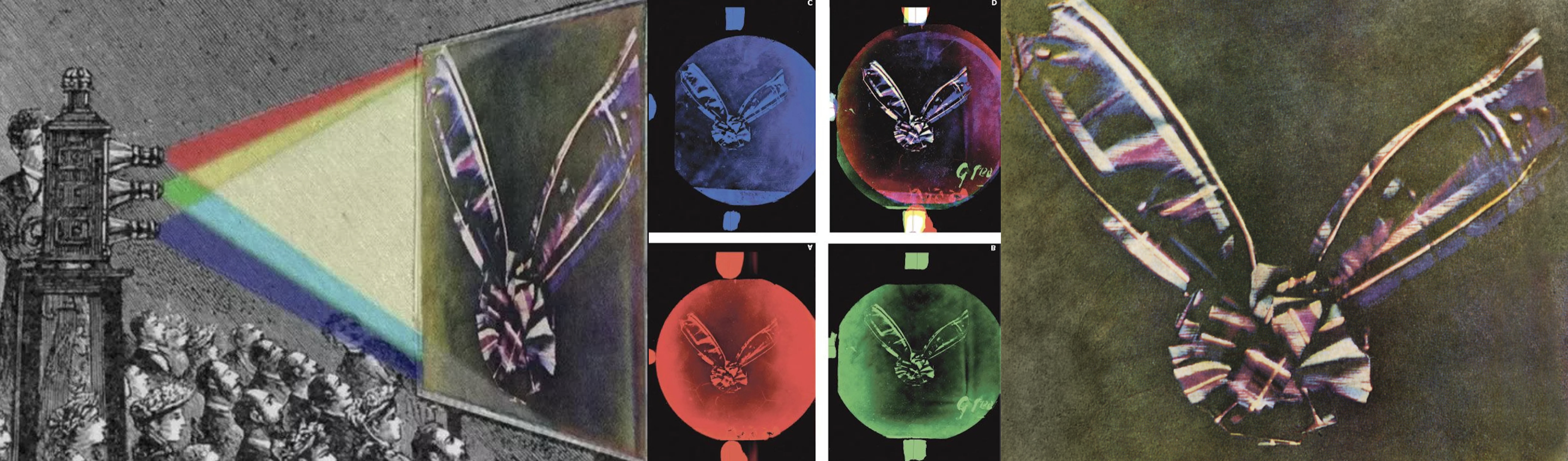
Maxwell’s 1861 tartan-ribbon experiment and its result. The ribbon was captured as three black-and-white plates, each shot through a red, green, or blue filter; projecting the three back through the same three colours and overlapping them reconstructs a recognisable colour image (centre), reproduced at right — the first colour photograph, conjured from grey plates and coloured lamps. Each plate is a map of how much of one band the ribbon reflected.
There is an honest footnote owed here, because the demonstration is more famous than it is sound, and the story improves for the telling. The photographic emulsions of 1861 — wet collodion — were essentially blind to red light and only feebly sensitive to green. By rights the red plate should have come out blank, and the whole composite should have failed. It worked because of a coincidence nobody understood until the 1961 centenary, when R. M. Evans at Kodak reconstructed the experiment and found the culprit: many of the red dyes used in tartan are also strong reflectors of ultraviolet, and Sutton’s deep red filter passed a little near-UV, to which the collodion was sensitive. The “red” plate was in truth a near-ultraviolet plate, recording a band the eye cannot see, standing in by luck for the red the eye can. Maxwell got the right result for the wrong reason — a clean demonstration of a true principle, resting on an accident of dye chemistry he never knew was holding it up. The principle survived the accident, which is the part that matters: the reduction of any stimulus to three numbers is real, whatever filters happen to read them.
Maxwell came to this honestly, not as a stunt. He had been measuring colour since he was a student in Edinburgh, spinning a Newton-style colour top with sectors of coloured paper and reading off, on a scale around the rim, how much red and green and blue paper it took to match a grey. By 1855, five years before his work on electromagnetism, he had already stated in print the principle the ribbon would dramatise — that any colour the eye can see can be reproduced by a suitable mixture of three. The ribbon made the abstraction visible on a screen. What it did not do was explain why three numbers add up the way the eye needs them to. For that we have to leave London and go to a schoolmaster in Pomerania who never did a colour experiment in his life.
Grassmann in Stettin
Now to make this precise. The claim hidden inside Maxwell’s demonstration is that colour matching behaves linearly — that matches can be scaled and added like ordinary algebra — and that claim was isolated, stated cleanly, and turned into mathematics eight years before the ribbon, by a man working entirely from his armchair.
The occasion was a quarrel. In 1852 Hermann von Helmholtz had argued, from his own prism experiments, that only one pair of pure spectral colours — a yellow and an indigo — could be mixed to white. Grassmann thought this both wrong and beside the point, and in 1853 he published a rebuttal, “Zur Theorie der Farbenmischung,” in Poggendorff’s Annalen der Physik. He did no new experiments. He simply wrote down the handful of facts about colour mixing that any careful observer already agreed on, and showed that Newton’s old doctrine — that every spectral colour has a complement that whites it out — followed from them by pure deduction. The facts he leaned on are now called Grassmann’s laws, and read in modern eyes they are not really laws about colour at all. They are the axioms of a vector space, with colour as the example.
Write to mean “the test light is judged an exact visual match to a mixture of units of primary , of , and of .” The relation is “looks identical to.” The empirical content of Grassmann’s laws is four statements about how behaves.
Read that list again with a linear-algebra eye and the disguise falls away. Lights superpose by addition — shine two together and their spectral powers add, — and they scale by a non-negative dimmer knob, . So the physical lights form a positive cone: closed under addition and under non-negative scaling, but with no way to subtract, since no lamp emits negative light. Grassmann’s laws 3 and 4 say that the matching relation respects exactly these two operations. The proof that this forces a vector-space structure is short enough to give in full.
The one thing needing care is that the operations are well defined on classes — that the answer does not depend on which representative light you pick out of a class. That is precisely what additivity buys. If and , then applying additivity twice gives , so does not depend on the representatives; scaling does the same job for . With addition and scaling well defined, is a commutative monoid with a scaling action — an algebraic positive cone. To get a genuine vector space, with subtraction, we play the standard trick for turning a cancellative monoid into a group: the Grothendieck completion, forming formal differences exactly as the integers are built from the naturals or the rationals from the integers. Define
read as the formal colour ” minus ,” and check that addition and scaling pass to the quotient. The result is a real vector space. Physical lights sit inside it as the differences — the colours you can actually shine — and the rest of , the formal differences and their combinations, are negative colours: things you cannot emit, but can perfectly well subtract. We are about to need them.
This is the abstract skeleton. The flesh comes from physiology, and it explains why the dimension is three and not seventeen. Recall the cone-response map of Post 2: each cone class integrates the incoming spectrum against its own sensitivity curve,
Each of these is a linear functional of the spectrum: integration against a fixed curve is linear, so the cone map automatically satisfies and . Two lights match — excite all three cones identically — exactly when their difference lies in the common kernel of the three functionals, which was our definition of a match in Post 2. Grassmann’s laws are then not a mystery to be explained but an immediate corollary of linearity of the integral. The match classes are the level sets of the map , the colour vector space is canonically , and trichromacy — the empirical fact that three primaries suffice — is the single statement that the map has rank exactly three. Grassmann, in 1853, had the algebra without the cones; he proved the laws forced a three-dimensional space and could only say the dimension was an experimental fact. He had no idea there were three pigments at the back of the eye waiting to supply the reason. The axiomatic argument and the physiological one are the same argument, met from opposite ends seventy years apart.
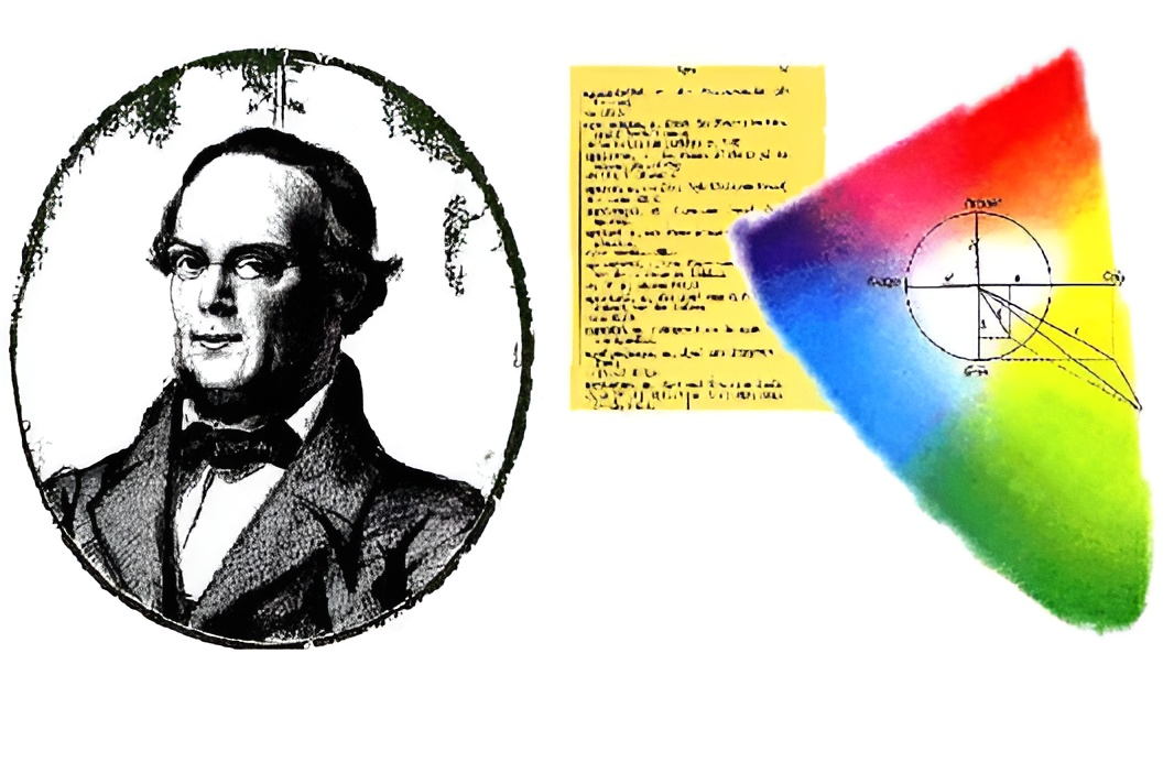
Hermann Grassmann (1809–1877), Gymnasium teacher in Stettin, whose 1853 paper on colour mixing was the only part of his mathematics understood in his lifetime — and which, read with a modern eye, states the axioms of a real vector space with colour as its first physical instance.
One subtlety deserves a remark, because the series will return to it. The reading of Grassmann’s laws as vector-space axioms is itself a modelling choice, made rigorous only in 1975 by David Krantz’s representation theorem, which shows the axioms (plus a regularity condition) force a canonical, coordinate-free homomorphism into a real vector space.
Where it holds, and where it bends
It would be a kind of lie to leave the laws standing as theorems, because they are not theorems about the eye — they are very good empirical approximations, and a careful book says where the approximation frays. Grassmann’s laws are physics-grade: accurate enough that every camera, display, and colour standard is built on them and works, and yet measurably false at the margins.
The additivity law is the one under most strain. It assumes the response to a sum of lights is the sum of the responses, but the visual system adapts to its own input — the gain on each cone channel drifts with the overall light level and its spectral makeup — so at very high luminances, and again at very low ones where the rods of the last post intrude on a supposedly cone-only match, the clean additivity of develops a wobble. Transitivity, too, has been shown to fail slightly for matches made at short wavelengths in the deep blue, where the numbers can drift by a few just-noticeable differences. And there is a famous effect, the Helmholtz–Kohlrausch phenomenon, in which a vividly saturated light looks brighter than a white of the same measured luminance — a real nonlinearity of perceived brightness, though one that touches the brightness reckoning rather than the matching relation itself, so it bends the eye without formally breaking the law.
None of this is fatal, and it is important to be clear why. The deviations are small, structured, and mostly confined to extremes of intensity and saturation that ordinary scenes rarely reach. They will matter later — when we meet displays with very narrow-band primaries, where two observers’ slightly different cone curves make a match for one a visible mismatch for the other, the small print of Post 3’s “match to me” cashed out in hardware. For the geometry we are building now, the laws hold to the precision the geometry needs. The honest statement is the one the style of this whole subject demands: colour matching is linear, to engineering tolerance, and the places it is not are themselves orderly enough to study.
Three numbers, made rigorous
We have been saying “the spectrum collapses to three numbers” since Post 1, and it is time to give that sentence its full mathematical weight, because the rest of the series lives inside the picture it draws.
A light, physically, is a spectral power distribution: a function assigning a non-negative power to each wavelength across the visible band. The natural home for such objects is a function space — take , square-integrable on the visible interval — which is infinite-dimensional. There is no finite list of numbers that pins down an arbitrary spectrum; you would need the value at every one of a continuum of wavelengths. This is the true size of the input. A sodium lamp’s near-spike at , the smooth hump of an incandescent bulb, the jagged comb of a fluorescent tube, the broad reflection of a leaf — all distinct points in an infinite-dimensional space, all carrying, in principle, unboundedly much information about the light.
The eye applies three linear functionals to this space and keeps only their three values. On each functional is an inner product against a fixed sensitivity curve,
which is exactly the integral form of rewritten as projection. The map
is a bounded linear surjection from an infinite-dimensional space onto a three-dimensional one. That single arrow is the whole subject in miniature, and almost every difficulty in the series is a property of it. Its kernel is enormous — an infinite-dimensional subspace of spectra that the eye reads as identical to darkness, and whose cosets are the metamer classes: two lights match precisely when they differ by an element of . Metamerism is not a quirk; it is the generic consequence of projecting an infinite-dimensional space onto a three-dimensional one, the inevitable crowd of pre-images sitting over every point of the image.
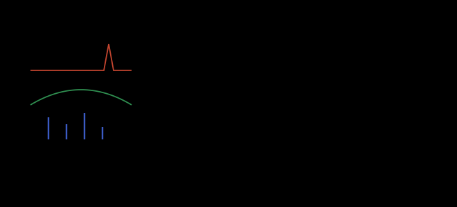
The colour map as a projection: the infinite-dimensional space of spectra , drawn as a function plotted over wavelength, sent by three inner products to a single point in . The fibres over each point — whole infinite-dimensional families of spectra collapsing to the same triple — are the metamer classes; the choice of three basis vectors in the target (cone fundamentals, RGB primaries, or XYZ) is what names the axes.
The choice of which three curves to integrate against is exactly a choice of basis in the target . Integrate against the cone fundamentals and you get the coordinates of Post 2. Integrate against Maxwell’s three filter responses and you get RGB coordinates. The two are related by an invertible matrix — a change of basis — because they are different bases of the same three-dimensional image of . This is why Maxwell’s reproduction works at all, restated with the algebra showing: his filter-and-plate triple spans the same three-dimensional subspace of spectral responses that the cones span, so any spectrum and its three-number reproduction sit in the same fibre of , hence in the same metamer class, hence visually identical. RGB, LMS, and the XYZ we are about to build are three coordinate systems on one three-dimensional space — the same room, measured against different walls. Keep that picture fixed and every transform in the rest of the series is just a matrix carrying one set of axes to another.
The negative lobe
Here is where the clean picture acquires its first crack, and the crack is the reason the next post exists.
Maxwell’s principle promises that three primaries can match any colour. The promise needs testing, and the test is the colour-matching experiment, the experiment that turned “three numbers” from a slogan into a measured set of curves. The protocol is simple to describe. An observer looks at a small circular field, split across the middle into two half-discs. One half shows a pure spectral test light at a chosen wavelength . The other half shows an additive mixture of three fixed primary lights, whose intensities the observer can turn up and down with three knobs. The task is to adjust the three primaries until the mixture half is indistinguishable from the test half — until the dividing line between them vanishes. The three knob settings that achieve the match, recorded as a function of the test wavelength and normalised per unit of test power, are the colour-matching functions , , .
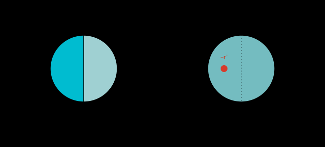
The bipartite matching field. A small circular target is split across a diameter: one half is a pure spectral test light, the other an additive mixture of three primaries the observer controls. A match is declared when the seam between the halves disappears. For cyan-green test lights no positive mixture suffices, and the only way to close the match is to move one primary — the red — across to the test side, recording it as a negative coefficient.
This is precisely the experiment that fixed the modern standard. Between 1928 and 1929 W. David Wright, then a graduate student at Imperial College, ran it on ten observers; around 1930 John Guild at the National Physical Laboratory ran a version on seven more. Their seventeen pairs of eyes, reconciled onto a common set of primaries and averaged, became the CIE 1931 standard observer at a meeting in Cambridge in September 1931. The primaries they settled on are worth quoting exactly, since the negative lobe lives on them and we will carry these numbers forward.
Now to the crack. Run the experiment with a test light in the cyan-green, somewhere around to , and the observer discovers something the clean theory did not advertise: no setting of the three knobs works. Turn them however you like — all the green you have, blue and red trimmed to taste — and the mixture half stays stubbornly more washed-out, more pastel, than the vivid spectral cyan in the test half. The mixture is always too desaturated. You cannot reach the test colour by adding primaries, because every mixture of three real lights, all of them at least slightly broad in their effect on the cones, is less pure than a single spectral line.
The fix the experimenters found is the heart of the whole matter. If you cannot make the mixture more saturated, you can make the test less saturated, by the same amount — and you do that by taking one of the primaries, the red, and shining it not on the mixture side but on the test side, alongside the cyan. A touch of red light added to the cyan-green desaturates it, pulls it toward white, until it drops down to meet the dulled mixture the other two primaries can produce. The match is achieved. But the bookkeeping is now unavoidable: the red that should have been part of the mixture is on the opposite side of the equation. Move it back across algebraically and it arrives with a minus sign. The recorded coefficient is negative:
This is the negative lobe — a broad dip in across the cyan-greens where the red-matching function goes frankly below zero. It is not a measurement error or an artefact of the apparatus. It is forced by geometry, and the function space of the last section says exactly why. The three real primaries span a triangle of reachable chromaticities; the spectral colours, being the purest the eye can register, lie outside that triangle along the cyan-green flank. To name a colour outside the triangle in terms of the triangle’s corners, at least one coordinate must be negative — there is no other way to point past the edge of a triangle using its own vertices. The negative colours we built by Grothendieck completion a few sections ago, the formal differences that no lamp can emit, are not a mathematical indulgence after all. The colour-matching experiment hands you one directly, every time the test light is a saturated cyan.
The interaction below is the experiment itself, made operable. Sweep the test wavelength down into the cyan-green and watch the red knob refuse to help — then let it cross over.
W-09 — colour matching & the negative lobe. Drag the test-wavelength slider, or set the three primary sliders by hand to chase a match; the auto-match toggle solves for the CIE 1931 RGB amounts directly. As the test crosses into the cyan-greens near the red coefficient goes negative, and the bipartite field moves the red primary across to the test half — the only physical way to spend a negative amount of a light you cannot emit negatively. The plot traces the three matching functions live, with the negative lobe of dipping below the axis. Primaries: .
The static companion below shows the three functions whole, so the lobe can be read in one glance rather than discovered a wavelength at a time.
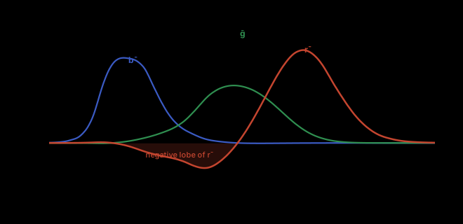
The CIE 1931 RGB colour-matching functions , , on the primaries, plotted across the visible band. The negative lobe of — the broad excursion below zero through the cyan-greens, roughly to — is shaded: these are the wavelengths at which matching demands a negative amount of red, i.e. red added to the test side. A static companion to W-09.
So the experiment that was supposed to confirm the tidy story instead complicates it. Three primaries do not match every colour by positive mixture; the matching functions dip below zero, and a colour space whose own basis vectors require negative coordinates to express real, visible, everyday spectral colours is an awkward thing to compute with and an embarrassing thing to standardise. You cannot build a colorimeter that emits negative light. You cannot tabulate a colour atlas in coordinates that go negative for half the spectrum without endless sign-juggling. The negativity is a genuine problem, and it was felt as one in 1931.
The solution the CIE reached for is as audacious as it is elegant, and it is the subject of the next post. If no triangle of real primaries can enclose the spectral colours, then choose primaries that are not real — three imaginary primaries, lying outside the spectrum locus entirely, deliberately impossible to emit, positioned so that their triangle swallows every colour the eye can see. The matching functions on those primaries never go negative. The price is that the primaries themselves correspond to no physical light: you trade real primaries with negative coordinates for impossible primaries with positive ones. That trade is the construction of the CIE XYZ system, and the negative lobe you just watched cross the field is exactly the thing it was engineered to cure.
Next: the horseshoe, and the three imaginary primaries that banish the negative lobe.